Model monitoring and drift detection
Contents
Model monitoring and drift detection#
This tutorial illustrates leveraging the model monitoring capabilities of MLRun to deploy a model to a live endpoint and calculate data drift.
Make sure you have reviewed the basics in MLRun Quick Start Tutorial.
Tutorial steps:
MLRun installation and configuration#
Before running this notebook make sure mlrun is installed and that you have configured the access to the MLRun service.
# Install MLRun if not installed, run this only once (restart the notebook after the install !!!)
%pip install mlrun
Set up the project#
First, import the dependencies and create an MLRun project. This contains all of the models, functions, datasets, etc:
import os

import mlrun
import pandas as pd
project = mlrun.get_or_create_project(name="tutorial", context="./", user_project=True)
> 2022-09-21 08:58:03,005 [info] loaded project tutorial from MLRun DB
Note
This tutorial does not focus on training a model. Instead, it starts with a trained model and its corresponding training dataset.
Next, log the following model file and dataset to deploy and calculate data drift. The model is a AdaBoostClassifier from sklearn, and the dataset is in csv format.
model_path = mlrun.get_sample_path('models/model-monitoring/model.pkl')
training_set_path = mlrun.get_sample_path('data/model-monitoring/iris_dataset.csv')
Log the model with training data#
Log the model using MLRun experiment tracking. This is usually done in a training pipeline, but you can also bring in your pre-trained models from other sources. See Working with data and model artifacts and Automated experiment tracking for more information.
model_name = "RandomForestClassifier"
model_artifact = project.log_model(
    key=model_name,
    model_file=model_path,
    framework="sklearn",
    training_set=pd.read_csv(training_set_path),
    label_column="label"
)
# the model artifact unique URI
model_artifact.uri
'store://models/tutorial-nick/RandomForestClassifier#0:latest'
Import and deploy the serving function#
Import the model server function from the MLRun Function Hub. Additionally, mount the filesytem, add the model that was logged via experiment tracking, and enable drift detection.
The core line here is serving_fn.set_tracking() that creates the required infrastructure behind the scenes to perform drift detection. See the Model monitoring overview for more info on what is deployed.
# Import the serving function from the Function Hub and mount filesystem
serving_fn = mlrun.import_function('hub://v2_model_server', new_name="serving")

# Add the model to the serving function's routing spec
serving_fn.add_model(model_name, model_path=model_artifact.uri)

# Enable model monitoring
serving_fn.set_tracking()
Deploy the serving function with drift detection#
Deploy the serving function with drift detection enabled with a single line of code:
mlrun.deploy_function(serving_fn)
> 2022-09-21 08:58:08,053 [info] Starting remote function deploy
2022-09-21 08:58:09  (info) Deploying function
2022-09-21 08:58:09  (info) Building
2022-09-21 08:58:10  (info) Staging files and preparing base images
2022-09-21 08:58:10  (info) Building processor image
2022-09-21 08:58:55  (info) Build complete
2022-09-21 08:59:03  (info) Function deploy complete
> 2022-09-21 08:59:04,232 [info] successfully deployed function: {'internal_invocation_urls': ['nuclio-tutorial-nick-serving.default-tenant.svc.cluster.local:8080'], 'external_invocation_urls': ['tutorial-nick-serving-tutorial-nick.default-tenant.app.us-sales-350.iguazio-cd1.com/']}
DeployStatus(state=ready, outputs={'endpoint': 'http://tutorial-nick-serving-tutorial-nick.default-tenant.app.us-sales-350.iguazio-cd1.com/', 'name': 'tutorial-nick-serving'})
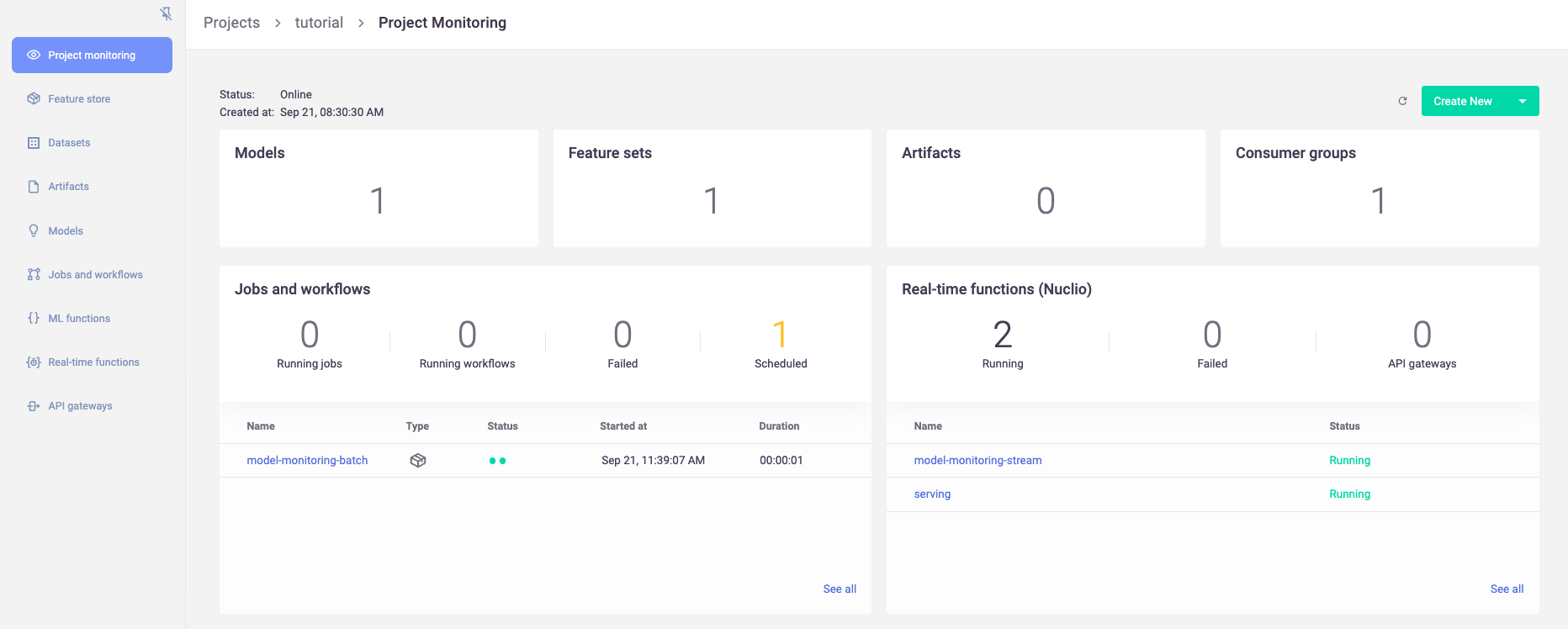
View deployed resources#
At this point, you should see the newly deployed model server, as well as a model-monitoring-stream, and a scheduled job (in yellow). The model-monitoring-stream collects, processes, and saves the incoming requests to the model server. The scheduled job does the actual calculation (by default every hour).
Note
You will not see model-monitoring-batch jobs listed until they actually run (by default every hour).
Simulate production traffic#
Next, use the following code to simulate incoming production data using elements from the training set. Because the data is coming from the same training set you logged, you should not expect any data drift.
Note
By default, the drift calculation starts via the scheduled hourly batch job after receiving 10,000 incoming requests.
import json
import logging
from random import choice, uniform
from time import sleep

from tqdm import tqdm

# Suppress print messages
logging.getLogger(name="mlrun").setLevel(logging.WARNING)

# Get training set as list
iris_data = pd.read_csv(training_set_path).drop("label", axis=1).to_dict(orient="split")["data"]

# Simulate traffic using random elements from training set
for i in tqdm(range(12_000)):
    data_point = choice(iris_data)
    serving_fn.invoke(f'v2/models/{model_name}/infer', json.dumps({'inputs': [data_point]}))

# Resume normal logging
logging.getLogger(name="mlrun").setLevel(logging.INFO)
100%|██████████| 12000/12000 [06:45<00:00, 29.63it/s]
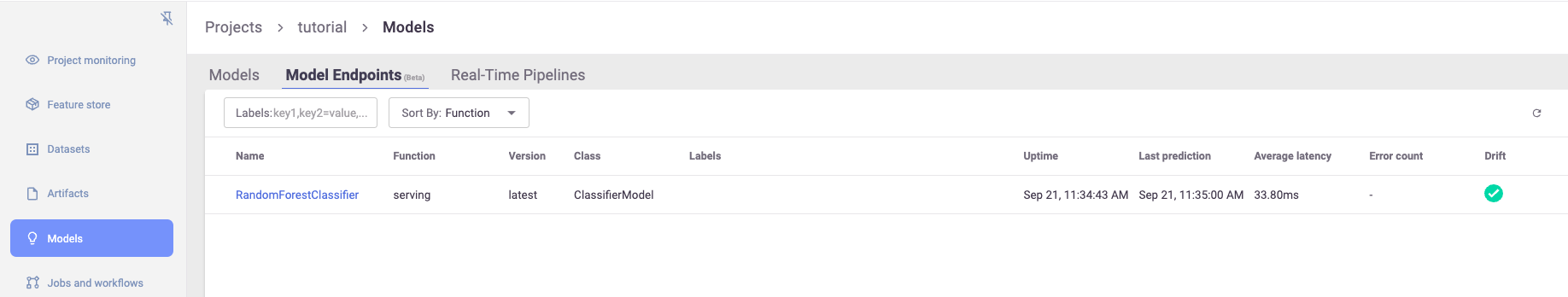
View drift calculations and status#
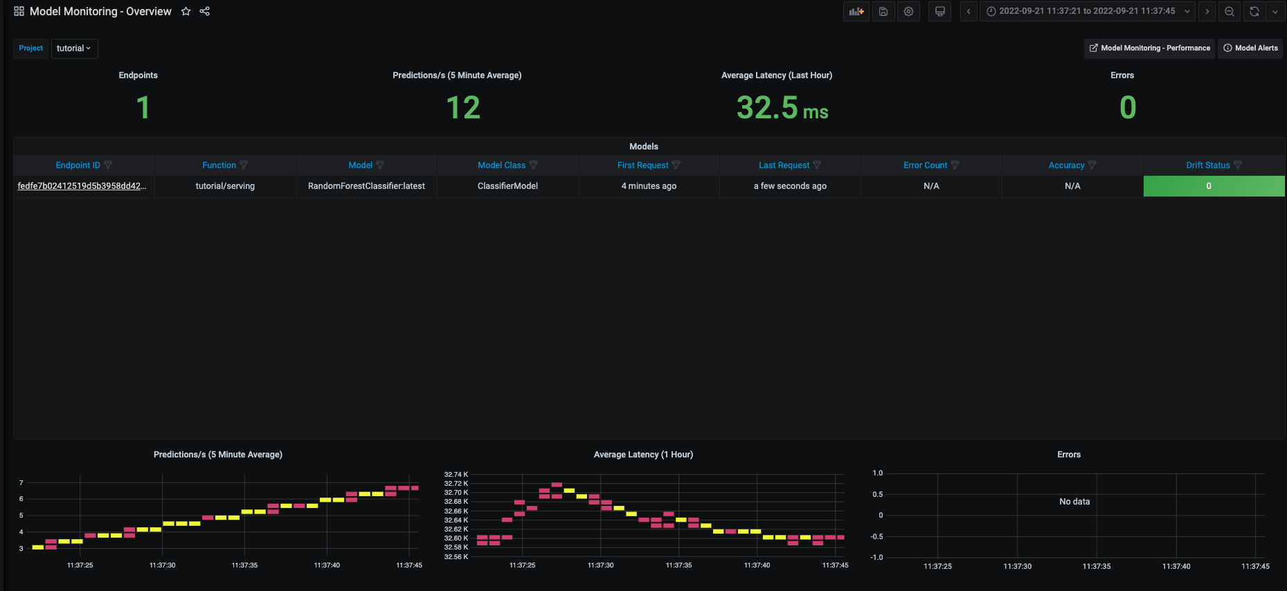
Once data drift has been calculated, you can view it in the MLRun UI. This includes a high level overview of the model status:
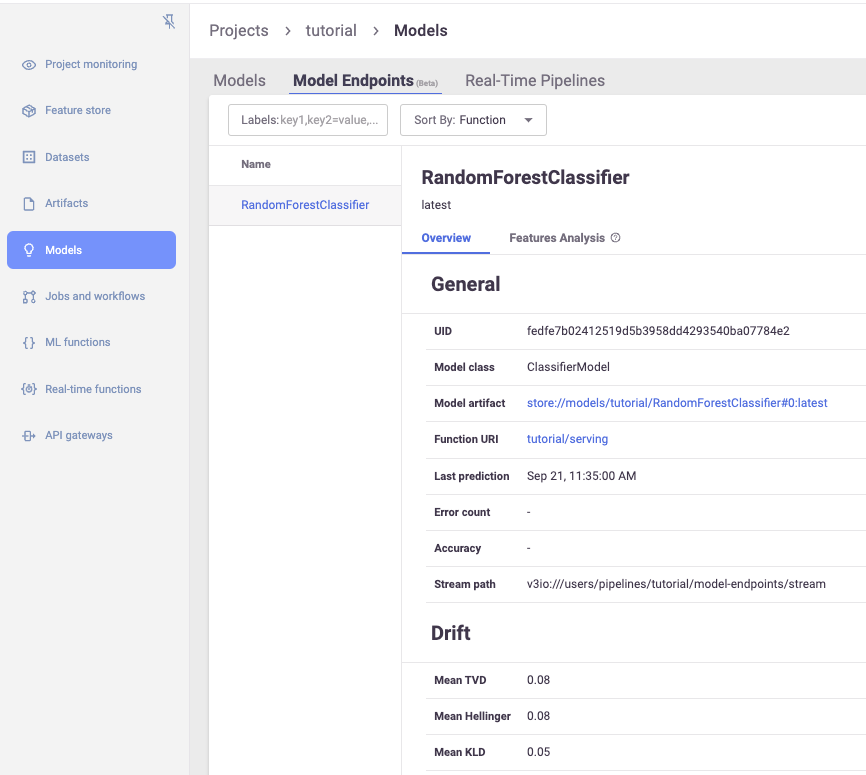
A more detailed view on model information and overall drift metrics:
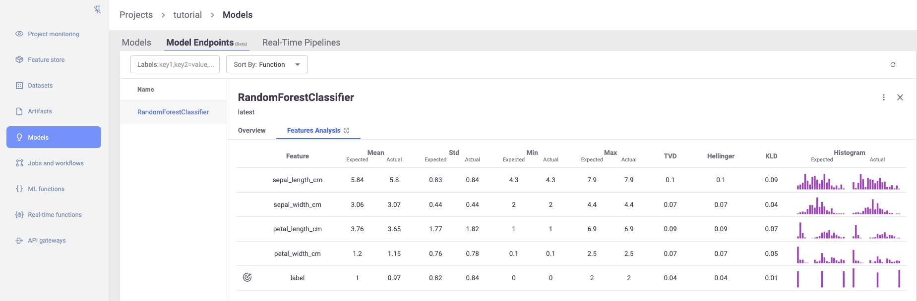
As well as a view for feature-level distributions and drift metrics:
View detailed drift dashboards#
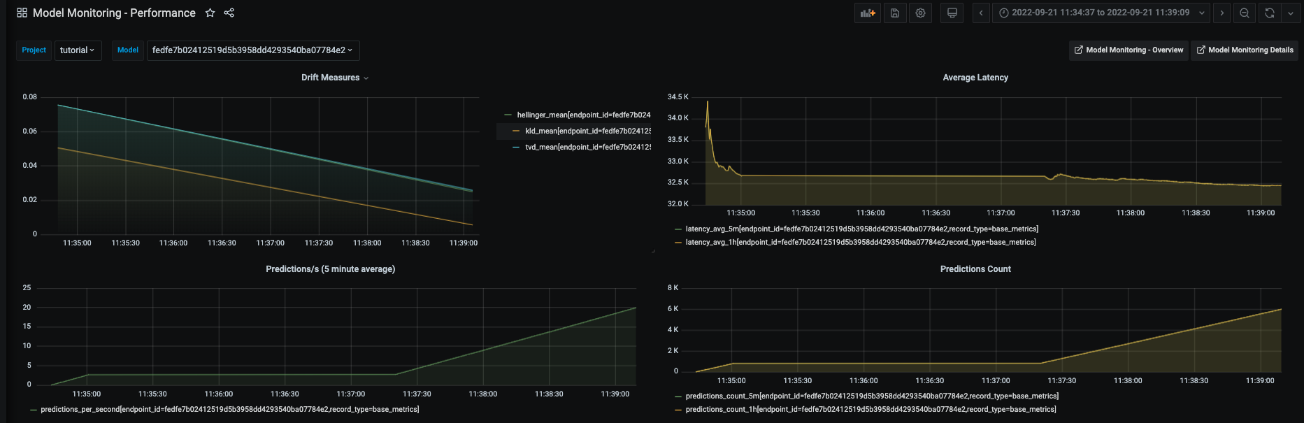
Finally, there are also more detailed Grafana dashboards that show additional information on each model in the project:
For more information on accessing these dashboards, see Model monitoring using Grafana dashboards.
Graphs of individual features over time:
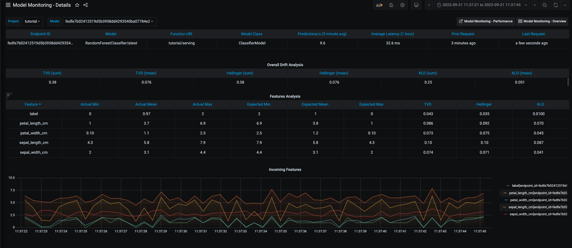
As well as drift and operational metrics over time: