
Batch inference and drift detection
Contents
Batch inference and drift detection#
This tutorial leverages a function from the MLRun Function Hub to perform batch inference using a logged model and a new prediction dataset. The function also calculates data drift by comparing the new prediction dataset with the original training set.
Make sure you have reviewed the basics in MLRun Quick Start Tutorial.
Tutorial steps:
MLRun installation and Configuration#
Before running this notebook make sure mlrun is installed and that you have configured the access to the MLRun service.
# Install MLRun if not installed, run this only once (restart the notebook after the install !!!)
%pip install mlrun
Set up a project#
First, import the dependencies and create an MLRun project. The project contains all of your models, functions, datasets, etc.:
import mlrun
import os
import pandas as pd
project = mlrun.get_or_create_project("tutorial", context="./", user_project=True)
> 2023-03-15 10:11:49,387 [info] loaded project tutorial from MLRun DB
Note
This tutorial does not focus on training a model. Instead, it starts with a trained model and its corresponding training and prediction dataset.
You will use the following model files and datasets to perform the batch prediction. The model is a DecisionTreeClassifier from sklearn and the datasets are in parquet format.
# We choose the correct model to avoid pickle warnings
import sys
suffix = mlrun.__version__.split("-")[0].replace(".", "_") if sys.version_info[1] > 7 else "3.7"

model_path = mlrun.get_sample_path(f'models/batch-predict/model-{suffix}.pkl')
training_set_path = mlrun.get_sample_path('data/batch-predict/training_set.parquet')
prediction_set_path = mlrun.get_sample_path('data/batch-predict/prediction_set.parquet')
View the data#
The training data has 20 numerical features and a binary (0,1) label:
pd.read_parquet(training_set_path).head()
| feature_0 | feature_1 | feature_2 | feature_3 | feature_4 | feature_5 | feature_6 | feature_7 | feature_8 | feature_9 | ... | feature_11 | feature_12 | feature_13 | feature_14 | feature_15 | feature_16 | feature_17 | feature_18 | feature_19 | label | |
|---|---|---|---|---|---|---|---|---|---|---|---|---|---|---|---|---|---|---|---|---|---|
| 0 | 0.572754 | 0.171079 | 0.403080 | 0.955429 | 0.272039 | 0.360277 | -0.995429 | 0.437239 | 0.991556 | 0.010004 | ... | 0.112194 | -0.319256 | -0.392631 | -0.290766 | 1.265054 | 1.037082 | -1.200076 | 0.820992 | 0.834868 | 0 |
| 1 | 0.623733 | -0.149823 | -1.410537 | -0.729388 | -1.996337 | -1.213348 | 1.461307 | 1.187854 | -1.790926 | -0.981600 | ... | 0.428653 | -0.503820 | -0.798035 | 2.038105 | -3.080463 | 0.408561 | 1.647116 | -0.838553 | 0.680983 | 1 |
| 2 | 0.814168 | -0.221412 | 0.020822 | 1.066718 | -0.573164 | 0.067838 | 0.923045 | 0.338146 | 0.981413 | 1.481757 | ... | -1.052559 | -0.241873 | -1.232272 | -0.010758 | 0.806800 | 0.661162 | 0.589018 | 0.522137 | -0.924624 | 0 |
| 3 | 1.062279 | -0.966309 | 0.341471 | -0.737059 | 1.460671 | 0.367851 | -0.435336 | 0.445308 | -0.655663 | -0.196220 | ... | 0.641017 | 0.099059 | 1.902592 | -1.024929 | 0.030703 | -0.198751 | -0.342009 | -1.286865 | -1.118373 | 1 |
| 4 | 0.195755 | 0.576332 | -0.260496 | 0.841489 | 0.398269 | -0.717972 | 0.810550 | -1.058326 | 0.368610 | 0.606007 | ... | 0.195267 | 0.876144 | 0.151615 | 0.094867 | 0.627353 | -0.389023 | 0.662846 | -0.857000 | 1.091218 | 1 |
5 rows × 21 columns
The prediciton data has 20 numerical features, but no label - this is what you will predict:
pd.read_parquet(prediction_set_path).head()
| feature_0 | feature_1 | feature_2 | feature_3 | feature_4 | feature_5 | feature_6 | feature_7 | feature_8 | feature_9 | feature_10 | feature_11 | feature_12 | feature_13 | feature_14 | feature_15 | feature_16 | feature_17 | feature_18 | feature_19 | |
|---|---|---|---|---|---|---|---|---|---|---|---|---|---|---|---|---|---|---|---|---|
| 0 | -2.059506 | -1.314291 | 2.721516 | -2.132869 | -0.693963 | 0.376643 | 3.017790 | 3.876329 | -1.294736 | 0.030773 | 0.401491 | 2.775699 | 2.361580 | 0.173441 | 0.879510 | 1.141007 | 4.608280 | -0.518388 | 0.129690 | 2.794967 |
| 1 | -1.190382 | 0.891571 | 3.726070 | 0.673870 | -0.252565 | -0.729156 | 2.646563 | 4.782729 | 0.318952 | -0.781567 | 1.473632 | 1.101721 | 3.723400 | -0.466867 | -0.056224 | 3.344701 | 0.194332 | 0.463992 | 0.292268 | 4.665876 |
| 2 | -0.996384 | -0.099537 | 3.421476 | 0.162771 | -1.143458 | -1.026791 | 2.114702 | 2.517553 | -0.154620 | -0.465423 | -1.723025 | 1.729386 | 2.820340 | -1.041428 | -0.331871 | 2.909172 | 2.138613 | -0.046252 | -0.732631 | 4.716266 |
| 3 | -0.289976 | -1.680019 | 3.126478 | -0.704451 | -1.149112 | 1.174962 | 2.860341 | 3.753661 | -0.326119 | 2.128411 | -0.508000 | 2.328688 | 3.397321 | -0.932060 | -1.442370 | 2.058517 | 3.881936 | 2.090635 | -0.045832 | 4.197315 |
| 4 | -0.294866 | 1.044919 | 2.924139 | 0.814049 | -1.455054 | -0.270432 | 3.380195 | 2.339669 | 1.029101 | -1.171018 | -1.459395 | 1.283565 | 0.677006 | -2.147444 | -0.494150 | 3.222041 | 6.219348 | -1.914110 | 0.317786 | 4.143443 |
Log the model with training data#
Next, log the model using MLRun experiment tracking. This is usually done in a training pipeline, but you can also bring in your pre-trained models from other sources. See Working with data and model artifacts and Automated experiment tracking for more information.
In this example, you are logging a training set with the model for future comparison, however you can also directly pass in your training set to the batch prediction function.
model_artifact = project.log_model(
    key="model",
    model_file=model_path,
    framework="sklearn",
    training_set=pd.read_parquet(training_set_path),
    label_column="label"
)
# the model artifact unique URI
model_artifact.uri
Import and run the batch inference function#
Next, import the batch inference function from the MLRun Function Hub:
fn = mlrun.import_function("hub://batch_inference")
Run batch inference#
Finally, perform the batch prediction by passing in your model and datasets. See the corresponding batch inference example notebook for an exhaustive list of other parameters that are supported:
run = project.run_function(
    fn,
    inputs={
        "dataset": prediction_set_path,
        # If you do not log a dataset with your model, you can pass it in here:
#       "sample_set" : training_set_path
    },
    params={
        "model": model_artifact.uri,
        "perform_drift_analysis" : True,
    },
)
> 2023-03-15 10:11:50,578 [info] starting run batch-inference-infer uid=b357c4bc6ccf48e8a18803bab02f919a DB=http://mlrun-api:8080
> 2023-03-15 10:11:50,802 [info] Job is running in the background, pod: batch-inference-infer-wzdcg
final state: completed
| project | uid | iter | start | state | name | labels | inputs | parameters | results | artifacts |
|---|---|---|---|---|---|---|---|---|---|---|
| tutorial-yonis | 0 | Mar 15 10:11:54 | completed | batch-inference-infer | v3io_user=yonis kind=job owner=yonis mlrun/client_version=1.2.1 host=batch-inference-infer-wzdcg |
dataset |
model=store://models/tutorial-yonis/model#0:69f79f68-b455-45d8-a461-9340fb64fb28 perform_drift_analysis=True |
batch_id=8616574bd1078ebdd43d2bf350d8d14321d2072dd969ebccc8c55afd drift_status=False drift_metric=0.31451973312099435 |
prediction drift_table_plot features_drift_results |
> 2023-03-15 10:12:03,958 [info] run executed, status=completed
View predictions and drift status#
These are the batch predictions on the prediction set from the model:
run.artifact("prediction").as_df().head()
| feature_0 | feature_1 | feature_2 | feature_3 | feature_4 | feature_5 | feature_6 | feature_7 | feature_8 | feature_9 | ... | feature_11 | feature_12 | feature_13 | feature_14 | feature_15 | feature_16 | feature_17 | feature_18 | feature_19 | label | |
|---|---|---|---|---|---|---|---|---|---|---|---|---|---|---|---|---|---|---|---|---|---|
| 0 | -2.059506 | -1.314291 | 2.721516 | -2.132869 | -0.693963 | 0.376643 | 3.017790 | 3.876329 | -1.294736 | 0.030773 | ... | 2.775699 | 2.361580 | 0.173441 | 0.879510 | 1.141007 | 4.608280 | -0.518388 | 0.129690 | 2.794967 | 0 |
| 1 | -1.190382 | 0.891571 | 3.726070 | 0.673870 | -0.252565 | -0.729156 | 2.646563 | 4.782729 | 0.318952 | -0.781567 | ... | 1.101721 | 3.723400 | -0.466867 | -0.056224 | 3.344701 | 0.194332 | 0.463992 | 0.292268 | 4.665876 | 1 |
| 2 | -0.996384 | -0.099537 | 3.421476 | 0.162771 | -1.143458 | -1.026791 | 2.114702 | 2.517553 | -0.154620 | -0.465423 | ... | 1.729386 | 2.820340 | -1.041428 | -0.331871 | 2.909172 | 2.138613 | -0.046252 | -0.732631 | 4.716266 | 0 |
| 3 | -0.289976 | -1.680019 | 3.126478 | -0.704451 | -1.149112 | 1.174962 | 2.860341 | 3.753661 | -0.326119 | 2.128411 | ... | 2.328688 | 3.397321 | -0.932060 | -1.442370 | 2.058517 | 3.881936 | 2.090635 | -0.045832 | 4.197315 | 0 |
| 4 | -0.294866 | 1.044919 | 2.924139 | 0.814049 | -1.455054 | -0.270432 | 3.380195 | 2.339669 | 1.029101 | -1.171018 | ... | 1.283565 | 0.677006 | -2.147444 | -0.494150 | 3.222041 | 6.219348 | -1.914110 | 0.317786 | 4.143443 | 0 |
5 rows × 21 columns
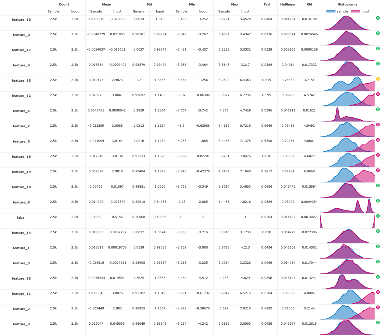
There is also a drift table plot that compares the drift between the training data and prediction data per feature:
run.artifact("drift_table_plot").show()
Finally, you also get a numerical drift metric and boolean flag denoting whether or not data drift is detected:
run.status.results
{'batch_id': '8616574bd1078ebdd43d2bf350d8d14321d2072dd969ebccc8c55afd',
 'drift_status': False,
 'drift_metric': 0.31451973312099435}
# Data/concept drift per feature
import json
json.loads(run.artifact("features_drift_results").get())
{'feature_14': 0.046364723781764774,
 'feature_10': 0.042567035578799796,
 'feature_1': 0.04485072701663093,
 'feature_2': 0.7391279921664593,
 'feature_0': 0.028086840976606773,
 'feature_17': 0.03587785749574268,
 'feature_8': 0.039060131873550404,
 'feature_13': 0.04239724655474124,
 'feature_15': 0.6329075683793959,
 'feature_19': 0.7902698698155215,
 'feature_9': 0.04468363504674985,
 'feature_16': 0.7181622588902428,
 'label': 0.33613674196785814,
 'feature_5': 0.05184219833790496,
 'feature_12': 0.7034787615778625,
 'feature_3': 0.043769819014849734,
 'feature_18': 0.04443732609382538,
 'feature_6': 0.7262042202197605,
 'feature_7': 0.7297906294873706,
 'feature_11': 0.7221431701127441,
 'feature_4': 0.042755641152500176}
Next steps#
In a production setting, you probably want to incorporate this as part of a larger pipeline or application.
For example, if you use this function for the prediction capabilities, you can pass the prediction output as the input to another pipeline step, store it in an external location like S3, or send to an application or user.
If you use this function for the drift detection capabilities, you can use the drift_status and drift_metrics outputs to automate further pipeline steps, send a notification, or kick off a re-training pipeline.