Feature set transformations#

A feature set contains an execution graph of operations that are performed when data is ingested, or when simulating data flow for inferring its metadata. This graph utilizes MLRun's Real-time serving pipelines (graphs).

The graph contains steps that represent data sources and targets, and may also contain steps whose purpose is transformations and enrichment of the data passed through the feature set. These transformations can be provided in one of three ways:

Aggregations — MLRun supports adding aggregate features to a feature set through the add_aggregation() function.
Built-in transformations — MLRun is equipped with a set of transformations provided through the storey.transformations package. These transformations can be added to the execution graph to perform common operations and transformations.
Custom transformations — You can extend the built-in functionality by adding new classes that perform any custom operation and use them in the serving graph.

Once a feature-set is created, its internal execution graph can be observed by calling the feature-set's plot() function, which generates a graphviz plot based on the internal graph. This is very useful when running within a Jupyter notebook, and produces a graph such as the following example:

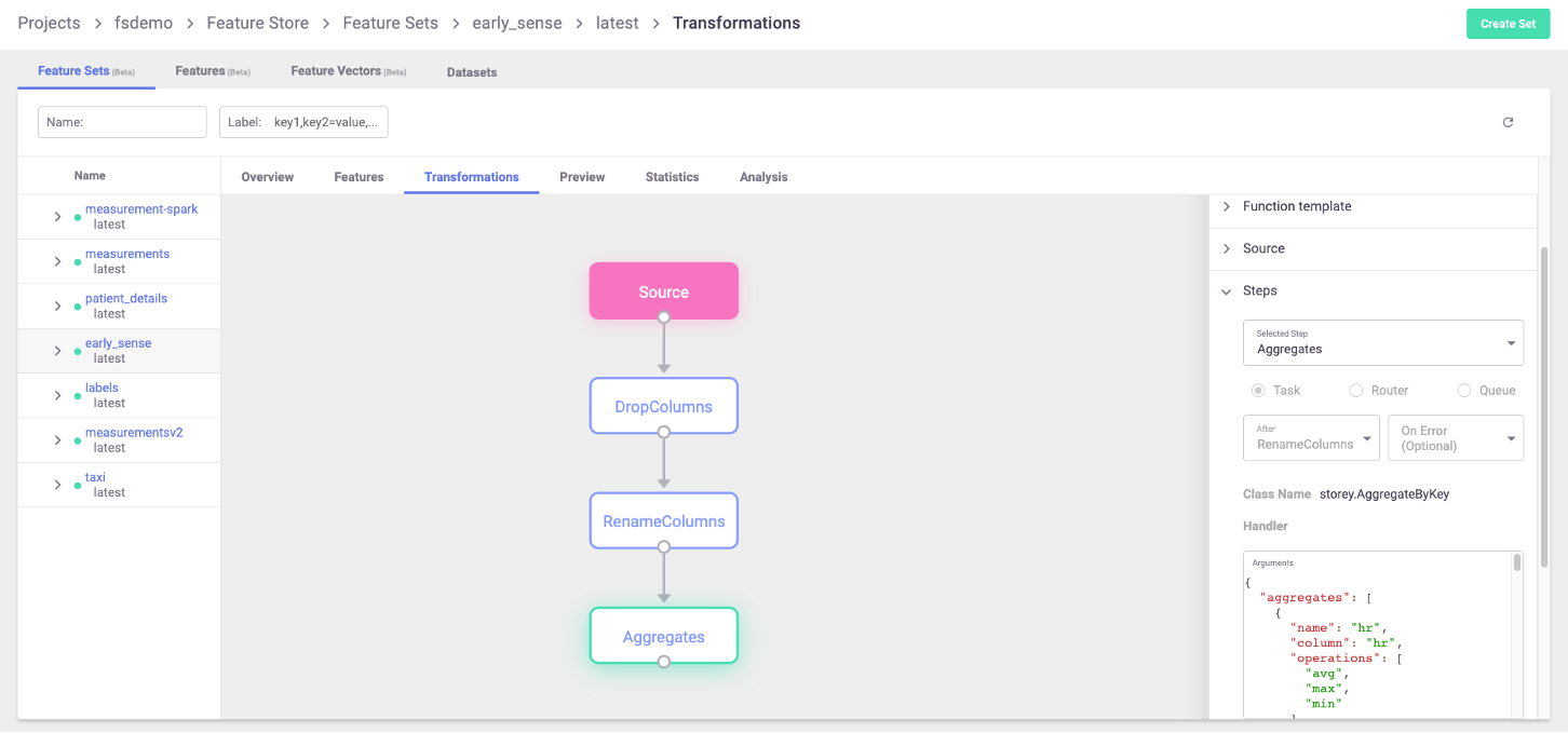
This plot shows various transformations and aggregations being used as part of the feature-set processing, as well as the targets where results are saved to (in this case two targets). Feature-sets can also be observed in the MLRun UI, where the full graph can be seen and specific step properties can be observed:

For a full end-to-end example of feature-store and usage of the functionality described in this page, refer to the feature store example.

In this section

Aggregations
Built-in transformations
Custom transformations
Data transformation steps

Aggregations#

Aggregations, being a common tool in data preparation and ML feature engineering, are available directly through the MLRun FeatureSet class. These transformations add a new feature to the feature-set, which is created by performing an aggregate function over the feature's values.

If the name parameter is not specified, features are generated in the format {column_name}_{operation}_{window}.
If you supply the optional name parameter, features are generated in the format {name}_{operation}_{window}.

Feature names, which are generated internally, must match this regex pattern to be treated as aggregations: .*_[a-z]+_[0-9]+[smhd]$,
where [a-z]+ is the name of an aggregation.

Warning

You must ensure that your features will not conflict with the automatically generated feature names. For example, when using add_aggregation() on a feature X, you may get a generated feature name of X_count_1h. But if your dataset already contains X_count_1h, this would result in either unreliable aggregations or errors.

If either the pattern or the condition is not met, the feature is treated as a static (or "regular") feature.

These features can be fed into predictive models or can be used for additional processing and feature generation.

Notes

Internally, the graph step that is created to perform these aggregations is named "Aggregates". If more than one aggregation steps are needed, a unique name must be provided to each, using the step_name parameter.
The timestamp column must be part of the feature set definition (for aggregation).

Aggregations that are supported using this function are:

count
sum
sqr (sum of squares)
max
min
first
last
avg
stdvar (variance)
stddev (standard deviation)

For full description of this function, see the add_aggregation() documentation.

Windows#

You can use aggregation for time-based sliding windows and fixed windows. In general, sliding windows are used for real time data, while fixed windows are used for historical aggregations.

A window can be measured in years, days, hours, seconds, minutes. A window can be a single window, e.g. ‘1h’, ‘1d’, or a list of same unit windows e.g. [‘1h’, ‘6h’]. If you define the time period (in addition to the window), then you have a sliding window. If you don't define the time period, then the time period and the window are the same. All time windows are aligned to the epoch (1970-01-01T00:00:00Z).

Sliding window

Sliding windows are fixed-size, overlapping, windows (defined by windows) that are evaluated at a sliding interval (defined by period).
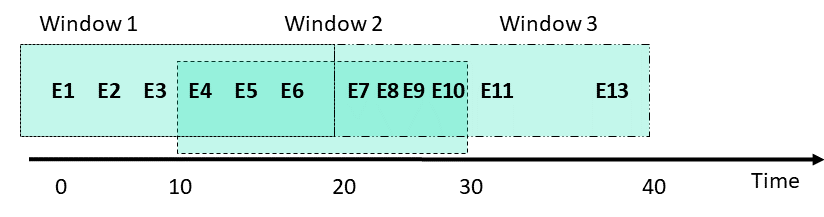
The period size must be an integral divisor of the window size.

The following figure illustrates sliding windows of size 20 seconds, and periods of 10 seconds. Since the period is less than the window size, the windows contain overlapping data. In this example, events E4-E6 are in Windows 1 and 2. When Window 2 is evaluated at time t = 30 seconds, events E4-E6 are dropped from the event queue.

The following code illustrates a feature-set that contains stock trading data including the specific bid price for each bid at any given time. You can add aggregate features that show the minimal and maximal bidding price over all the bids in the last 60 minutes, evaluated (sliding) at a 10 minute interval, per stock ticker (which is the entity in question).
```
import mlrun.feature_store as fstore
# create a new feature set
quotes_set = fstore.FeatureSet("stock-quotes", entities=[fstore.Entity("ticker")])
quotes_set.add_aggregation("bid", ["min", "max"], ["1h"], "10m", name="price")
```
This code generates two new features: bid_min_1h and bid_max_1h every 10 minutes.
Fixed window

A fixed window has a fixed-size, is non-overlapping, and gapless. A fixed time window is used for aggregating over a time period, (or day of the week). For example, how busy is a restaurant between 1 and 2 pm.
When using a fixed window, each record in an in-application stream belongs to a specific window. The record is processed only once (when the query processes the window to which the record belongs).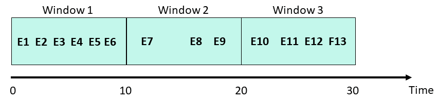

To define a fixed window, omit the time period. Using the above example, but for a fixed window:
```
import mlrun.feature_store as fstore
# create a new feature set
quotes_set = fstore.FeatureSet("stock-quotes", entities=[fstore.Entity("ticker")])
quotes_set.add_aggregation("bid", ["min", "max"], ["1h"] name="price")
```
This code generates two new features: bid_min_1h and bid_max_1h once per hour.

Built-in transformations#

MLRun, and the associated storey package, have a built-in library of transformation functions that can be applied as steps in the feature-set's internal execution graph. To add steps to the graph, reference them from the FeatureSet object by using the graph property. Then, new steps can be added to the graph using the functions in storey.transformations (follow the link to browse the documentation and the list of existing functions). The transformations are also accessible directly from the storey module.

See the built-in steps.

Note

Internally, MLRun makes use of functions defined in the storey package for various purposes. When creating a feature-set and configuring it with sources and targets, what MLRun does behind the scenes is to add steps to the execution graph that wraps methods and classes that perform the actions. When defining an async execution graph, storey classes are used. For example, when defining a Parquet data-target in MLRun, a graph step is created that wraps storey's ParquetTarget function.

To use a function:

Access the graph from the feature-set object, using the graph property.
Add steps to the graph using the various graph functions, such as to(). The function object passed to the step should point at the transformation function being used.

The following is an example for adding a simple filter to the graph, that drops any bid that is lower than 50USD:

quotes_set.graph.to("storey.Filter", "filter", _fn="(event['bid'] > 50)")

In the example above, the parameter _fn denotes a callable expression that is passed to the storey.Filter class as the parameter fn. The callable parameter can also be a Python function, in which case there's no need for parentheses around it. This call generates a step in the graph called filter that calls the expression provided with the event being propagated through the graph as the data is fed to the feature-set.

Custom transformations#

When a transformation is needed that is not provided by the built-in functions, new classes that implement transformations can be created and added to the execution graph. Such classes should extend the MapClass class, and the actual transformation should be implemented within their do() function, which receives an event and returns the event after performing transformations and manipulations on it. For example, consider the following code:

class MyMap(MapClass):
    def __init__(self, multiplier=1, **kwargs):
        super().__init__(**kwargs)
        self._multiplier = multiplier

    def do(self, event):
        event["multi"] = event["bid"] * self._multiplier
        return event

The MyMap class can then be used to construct graph steps, in the same way as shown above for built-in functions:

quotes_set.graph.add_step("MyMap", "multi", after="filter", multiplier=3)

This uses the add_step function of the graph to add a step called multi utilizing MyMap after the filter step that was added previously. The class is initialized with a multiplier of 3.

Supporting multiple engines#

MLRun supports multiple processing engines for executing graphs. These engines differ in the way they invoke graph steps. When implementing custom transformations, the code has to support all engines that are expected to run it.

Note

The vast majority of MLRun's built-in transformations support all engines. The support matrix is available here.

The following are the main differences between transformation steps executing on different engines:

storey - the step receives a single event (either as a dictionary or as an Event object, depending on whether full_event is configured for the step). The step is expected to process the event and return the modified event.
spark - the step receives a Spark dataframe object. Steps are expected to add their processing and calculations to the dataframe (either in-place or not) and return the resulting dataframe without materializing the data.
pandas - the step receives a Pandas dataframe, processes it, and returns the dataframe.

To support multiple engines, extend the MLRunStep class with a custom transformation. This class allows implementing engine-specific code by overriding the following methods: _do_storey(), _do_pandas() and _do_spark(). To add support for a given engine, the relevant do method needs to be implemented.

When a graph is executed, each step is a single instance of the relevant class that gets invoked as events flow through the graph. For spark and pandas engines, this only happens once per ingestion, since the entire data-frame is fed to the graph. For the storey engine the same instance's _do_storey() function will be invoked per input row. As the graph is initialized, this class instance can receive global parameters in its __init__ method that determines its behavior.

The following example class multiplies a feature by a value and adds it to the event. (For simplicity, data type checks and validations were omitted as well as needed imports.) Note that the class also extends StepToDict - this class implements generic serialization of graph steps to a python dictionary. This functionality allows passing instances of this class to graph.to() and graph.add_step():

class MultiplyFeature(StepToDict, MLRunStep):
    def __init__(self, feature: str, value: int, **kwargs):
        super().__init__(**kwargs)
        self._feature = feature
        self._value = value
        self._new_feature = f"{feature}_times_{value}"

    def _do_storey(self, event):
        # event is a single row represented by a dictionary
        event[self._new_feature] = event[self._feature] * self._value  
        return event

    def _do_pandas(self, event):
        # event is a pandas.DataFrame
        event[self._new_feature] = event[self._feature].multiply(self._value)
        return event

    def _do_spark(self, event):
        # event is a pyspark.sql.DataFrame
        return event.withColumn(self._new_feature, 
                                col(self._feature) * lit(self._value)
                                )

The following example uses this step in a feature-set graph with the pandas engine. This example adds a feature called number1_times_4 with the value of the number1 feature multiplied by 4. Note how the global parameters are passed when creating the graph step:

import mlrun.feature_store as fstore

feature_set = fstore.FeatureSet("fs-new", 
                                entities=[fstore.Entity("id")], 
                                engine="pandas",
                                )
# Adding multiply step, with specific parameters
feature_set.graph.to(MultiplyFeature(feature="number1", value=4))
df_pandas = feature_set.ingest(data)

Data transformation steps#

The following table lists the available data-transformation steps. The next table details the ingestion engines support of these steps.

Class name	Description	Storey	Spark	Pandas
`#mlrun.feature_store.FeatureSet.add_aggregation()`	Aggregates the data into the table object provided for later persistence, and outputs an event enriched with the requested aggregation features.	Y Not supported with online target SQLTarget	Y	N
`mlrun.feature_store.steps.DateExtractor()`	Extract a date-time component.	Y	N Supports part extract (ex. day_of_week) but does not support boolean (ex. is_leap_year)	Y
`mlrun.feature_store.steps.DropFeatures()`	Drop features from feature list.	Y	Y	Y
`mlrun.feature_store.steps.Imputer()`	Replace None values with default values.	Y	Y	Y
`mlrun.feature_store.steps.MapValues()`	Map column values to new values.	Y	Y	Y
`mlrun.feature_store.steps.OneHotEncoder()`	Create new binary fields, one per category (one hot encoded).	Y	Y	Y
`mlrun.feature_store.steps.SetEventMetadata()`	Set the event metadata (id, key, timestamp) from the event body.	Y	N	N
`mlrun.feature_store.steps.FeaturesetValidator()`	Validate feature values according to the feature set validation policy	Y	N	Y