
Batch inference and drift detection#
This tutorial leverages mlrun's serving-as-a-job feature to perform batch inference, using a logged model and a new prediction dataset. The function also calculates data drift by comparing the new prediction dataset with the original training set.
Make sure you have reviewed the basics in MLRun Quick Start Tutorial.
In this tutorial
MLRun installation and configuration#
Before running this notebook make sure mlrun is installed and that you have configured the access to the MLRun service.
# Install MLRun if not installed, run this only once (restart the notebook after the install !!!)
%pip install mlrun
Set up a project#
First, import the dependencies and create an MLRun project. The project contains all of your models, functions, datasets, etc.:
import mlrun
import pandas as pd

project = mlrun.get_or_create_project(
    "tutorial", context="./", user_project=True, allow_cross_project=True
)
Note
This tutorial does not focus on training a model. Instead, it starts with a trained model and its corresponding training and prediction dataset.
You'll use the following model files and datasets to perform the batch prediction. The model is a DecisionTreeClassifier from sklearn and the datasets are in parquet format.
# Choose the correct model to avoid pickle warnings

suffix = mlrun.__version__.split("-")[0].replace(".", "_")

model_path = mlrun.get_sample_path(f"models/batch-predict/model-{suffix}.pkl")
training_set_path = mlrun.get_sample_path("data/batch-predict/training_set.parquet")
prediction_set_path = mlrun.get_sample_path("data/batch-predict/prediction_set.parquet")
drifted_prediction_set_path = mlrun.get_sample_path(
    "data/batch-predict/drifted_prediction_set.parquet"
)
View the data#
The training data has 20 numerical features and a binary (0,1) label:
pd.read_parquet(training_set_path).head()
| feature_0 | feature_1 | feature_2 | feature_3 | feature_4 | feature_5 | feature_6 | feature_7 | feature_8 | feature_9 | ... | feature_11 | feature_12 | feature_13 | feature_14 | feature_15 | feature_16 | feature_17 | feature_18 | feature_19 | label | |
|---|---|---|---|---|---|---|---|---|---|---|---|---|---|---|---|---|---|---|---|---|---|
| 0 | 0.572754 | 0.171079 | 0.403080 | 0.955429 | 0.272039 | 0.360277 | -0.995429 | 0.437239 | 0.991556 | 0.010004 | ... | 0.112194 | -0.319256 | -0.392631 | -0.290766 | 1.265054 | 1.037082 | -1.200076 | 0.820992 | 0.834868 | 0 |
| 1 | 0.623733 | -0.149823 | -1.410537 | -0.729388 | -1.996337 | -1.213348 | 1.461307 | 1.187854 | -1.790926 | -0.981600 | ... | 0.428653 | -0.503820 | -0.798035 | 2.038105 | -3.080463 | 0.408561 | 1.647116 | -0.838553 | 0.680983 | 1 |
| 2 | 0.814168 | -0.221412 | 0.020822 | 1.066718 | -0.573164 | 0.067838 | 0.923045 | 0.338146 | 0.981413 | 1.481757 | ... | -1.052559 | -0.241873 | -1.232272 | -0.010758 | 0.806800 | 0.661162 | 0.589018 | 0.522137 | -0.924624 | 0 |
| 3 | 1.062279 | -0.966309 | 0.341471 | -0.737059 | 1.460671 | 0.367851 | -0.435336 | 0.445308 | -0.655663 | -0.196220 | ... | 0.641017 | 0.099059 | 1.902592 | -1.024929 | 0.030703 | -0.198751 | -0.342009 | -1.286865 | -1.118373 | 1 |
| 4 | 0.195755 | 0.576332 | -0.260496 | 0.841489 | 0.398269 | -0.717972 | 0.810550 | -1.058326 | 0.368610 | 0.606007 | ... | 0.195267 | 0.876144 | 0.151615 | 0.094867 | 0.627353 | -0.389023 | 0.662846 | -0.857000 | 1.091218 | 1 |
5 rows × 21 columns
The prediction data has 20 numerical features, but no label - this is what you will predict:
pd.read_parquet(prediction_set_path).head()
| feature_0 | feature_1 | feature_2 | feature_3 | feature_4 | feature_5 | feature_6 | feature_7 | feature_8 | feature_9 | feature_10 | feature_11 | feature_12 | feature_13 | feature_14 | feature_15 | feature_16 | feature_17 | feature_18 | feature_19 | |
|---|---|---|---|---|---|---|---|---|---|---|---|---|---|---|---|---|---|---|---|---|
| 0 | -2.059506 | -1.314291 | 2.721516 | -2.132869 | -0.693963 | 0.376643 | 3.017790 | 3.876329 | -1.294736 | 0.030773 | 0.401491 | 2.775699 | 2.361580 | 0.173441 | 0.879510 | 1.141007 | 4.608280 | -0.518388 | 0.129690 | 2.794967 |
| 1 | -1.190382 | 0.891571 | 3.726070 | 0.673870 | -0.252565 | -0.729156 | 2.646563 | 4.782729 | 0.318952 | -0.781567 | 1.473632 | 1.101721 | 3.723400 | -0.466867 | -0.056224 | 3.344701 | 0.194332 | 0.463992 | 0.292268 | 4.665876 |
| 2 | -0.996384 | -0.099537 | 3.421476 | 0.162771 | -1.143458 | -1.026791 | 2.114702 | 2.517553 | -0.154620 | -0.465423 | -1.723025 | 1.729386 | 2.820340 | -1.041428 | -0.331871 | 2.909172 | 2.138613 | -0.046252 | -0.732631 | 4.716266 |
| 3 | -0.289976 | -1.680019 | 3.126478 | -0.704451 | -1.149112 | 1.174962 | 2.860341 | 3.753661 | -0.326119 | 2.128411 | -0.508000 | 2.328688 | 3.397321 | -0.932060 | -1.442370 | 2.058517 | 3.881936 | 2.090635 | -0.045832 | 4.197315 |
| 4 | -0.294866 | 1.044919 | 2.924139 | 0.814049 | -1.455054 | -0.270432 | 3.380195 | 2.339669 | 1.029101 | -1.171018 | -1.459395 | 1.283565 | 0.677006 | -2.147444 | -0.494150 | 3.222041 | 6.219348 | -1.914110 | 0.317786 | 4.143443 |
Log the model with training data#
Next, log the model using MLRun experiment tracking. This is usually done in a training pipeline, but you can also bring in your pre-trained models from other sources. See Working with data and model artifacts and Automated experiment tracking for more information.
In this example, you are logging a training set with the model for future comparison, however you can also directly pass in your training set to the batch prediction function.
model_path = "https://s3.wasabisys.com/iguazio/models/batch-predict/model-1_9_2.pkl"
model_artifact = project.log_model(
    key="model",
    model_file=model_path,
    framework="sklearn",
    training_set=pd.read_parquet(training_set_path),
    label_column="label",
)
# the model artifact unique URI
model_artifact.uri
Enabling model monitoring#
The MLRun's model monitoring service includes built-in model monitoring and reporting capabilities.
Visit MLRun's Model monitoring architecture to read more and check out the Model monitoring tutorial.
Modifying controller frequency with base_period parameter to 1 minute allows to see monitoring results faster, by default, its value is 10 minutes.
from src.model_monitoring_utils import enable_model_monitoring

# If this project was running with MM enabled pre-1.8.0, disable the old model monitoring to update configurations
project.disable_model_monitoring(delete_stream_function=True)

enable_model_monitoring(
    project=project,
    tsdb_profile_name="batch-tsdb",
    stream_profile_name="batch-stream",
    base_period=1,
    wait_for_deployment=True,
    deploy_histogram_data_drift_app=False,
)
Change the histogram data drift application defaults#
To generate the drift table plot artifact using MLRun's histogram data drift application, you have to change the application defaults.
You have to keep the default name of the application - "histogram-data-drift" - for its full functionality, including the statistics
that are used in the "Model Endpoint" -> "Feature Analysis" view in the UI.
import mlrun.model_monitoring.applications.histogram_data_drift as histogram_data_drift

custom_hist_app = project.set_model_monitoring_function(
    name=histogram_data_drift.HistogramDataDriftApplicationConstants.NAME,  # keep the default name
    func=histogram_data_drift.__file__,
    application_class=histogram_data_drift.HistogramDataDriftApplication.__name__,
    produce_json_artifact=True,
    produce_plotly_artifact=True,
)

project.deploy_function(custom_hist_app)
Create and run the serving job#
Next, set a serving function based on a custom class, add the model we logged earlier to its graph and convert the function to a job. Use the set_tracking method to enable monitoring of the model-endpoint.
import mlrun.common.schemas.model_monitoring.constants as mm_constants

fn = project.set_function(
    func="src/my_model.py", name="serving-fn-1", kind="serving", image="mlrun/mlrun"
)

graph = fn.set_topology("flow", engine="async")

model_runner_step = mlrun.serving.ModelRunnerStep(name="my_model_runner")

model_runner_step.add_model(
    model_class="MyModel",
    endpoint_name="my_model",
    model_artifact=model_artifact,
    execution_mechanism="naive",
    model_endpoint_creation_strategy=mm_constants.ModelEndpointCreationStrategy.OVERWRITE,
)

graph.to(model_runner_step).respond()
fn.set_tracking()
job = fn.to_job()
Run batch inference job#
Finally, perform the batch prediction by passing in your input dataset to the job you created and running it.
inputs = {"data": prediction_set_path}
run_obj = project.run_function(job, inputs=inputs)
> 2025-10-27 15:53:47,767 [info] Storing function: {"db":"http://mlrun-api:8080","name":"serving-fn-1-batch-execute-graph","uid":"ea36f45209894f10b68ad850b481eccc"}
> 2025-10-27 15:53:48,062 [info] Job is running in the background, pod: serving-fn-1-batch-execute-graph-ksptx
> 2025-10-27 15:53:51,653 [info] Waiting for model endpoint creation task '57b170c0-de5d-45cd-8bd2-571dd310eed6'...
> 2025-10-27 15:53:53,506 [info] Creating Model Monitoring stream target using uri:: {"uri":"ds://batch-stream/projects/tutorial-iguazio/model-endpoints/stream-v1"}
> 2025-10-27 15:53:53,524 [info] Initializing graph steps
> 2025-10-27 15:53:55,166 [info] Graph was initialized: {"verbose":false}
> 2025-10-27 15:54:01,554 [info] Job completed processing 2500 rows: {"model_endpoint_uids":["9a28537c8e364759b9178716d3d74287"],"timestamp_column":null}
> 2025-10-27 15:54:01,760 [info] To track results use the CLI: {"info_cmd":"mlrun get run ea36f45209894f10b68ad850b481eccc -p tutorial-iguazio","logs_cmd":"mlrun logs ea36f45209894f10b68ad850b481eccc -p tutorial-iguazio"}
> 2025-10-27 15:54:01,761 [info] Or click for UI: {"ui_url":"https://dashboard.default-tenant.app.vmdev219.lab.iguazeng.com/mlprojects/tutorial-iguazio/jobs/monitor-jobs/serving-fn-1-batch-execute-graph/ea36f45209894f10b68ad850b481eccc/overview"}
> 2025-10-27 15:54:01,761 [info] Run execution finished: {"name":"serving-fn-1-batch-execute-graph","status":"completed"}
| project | uid | iter | start | end | state | kind | name | labels | inputs | parameters | results | artifacts |
|---|---|---|---|---|---|---|---|---|---|---|---|---|
| tutorial-iguazio | 0 | Oct 27 15:53:51 | 2025-10-27 15:54:01.751376+00:00 | completed | run | serving-fn-1-batch-execute-graph | v3io_user=iguazio kind=job owner=iguazio mlrun/client_version=0.0.0+unstable mlrun/client_python_version=3.9.22 host=serving-fn-1-batch-execute-graph-ksptx |
data |
num_rows=2500 |
prediction |
> 2025-10-27 15:54:05,342 [info] Run execution finished: {"name":"serving-fn-1-batch-execute-graph","status":"completed"}
Predictions and drift status#
These are the batch predictions on the prediction set from the model:
run_obj.artifact("prediction").as_df().head()
| feature_0 | feature_1 | feature_2 | feature_3 | feature_4 | feature_5 | feature_6 | feature_7 | feature_8 | feature_9 | ... | feature_11 | feature_12 | feature_13 | feature_14 | feature_15 | feature_16 | feature_17 | feature_18 | feature_19 | label | |
|---|---|---|---|---|---|---|---|---|---|---|---|---|---|---|---|---|---|---|---|---|---|
| 0 | -2.059506 | -1.314291 | 2.721516 | -2.132869 | -0.693963 | 0.376643 | 3.017790 | 3.876329 | -1.294736 | 0.030773 | ... | 2.775699 | 2.361580 | 0.173441 | 0.879510 | 1.141007 | 4.608280 | -0.518388 | 0.129690 | 2.794967 | 1 |
| 1 | -1.190382 | 0.891571 | 3.726070 | 0.673870 | -0.252565 | -0.729156 | 2.646563 | 4.782729 | 0.318952 | -0.781567 | ... | 1.101721 | 3.723400 | -0.466867 | -0.056224 | 3.344701 | 0.194332 | 0.463992 | 0.292268 | 4.665876 | 0 |
| 2 | -0.996384 | -0.099537 | 3.421476 | 0.162771 | -1.143458 | -1.026791 | 2.114702 | 2.517553 | -0.154620 | -0.465423 | ... | 1.729386 | 2.820340 | -1.041428 | -0.331871 | 2.909172 | 2.138613 | -0.046252 | -0.732631 | 4.716266 | 0 |
| 3 | -0.289976 | -1.680019 | 3.126478 | -0.704451 | -1.149112 | 1.174962 | 2.860341 | 3.753661 | -0.326119 | 2.128411 | ... | 2.328688 | 3.397321 | -0.932060 | -1.442370 | 2.058517 | 3.881936 | 2.090635 | -0.045832 | 4.197315 | 0 |
| 4 | -0.294866 | 1.044919 | 2.924139 | 0.814049 | -1.455054 | -0.270432 | 3.380195 | 2.339669 | 1.029101 | -1.171018 | ... | 1.283565 | 0.677006 | -2.147444 | -0.494150 | 3.222041 | 6.219348 | -1.914110 | 0.317786 | 4.143443 | 0 |
5 rows × 21 columns
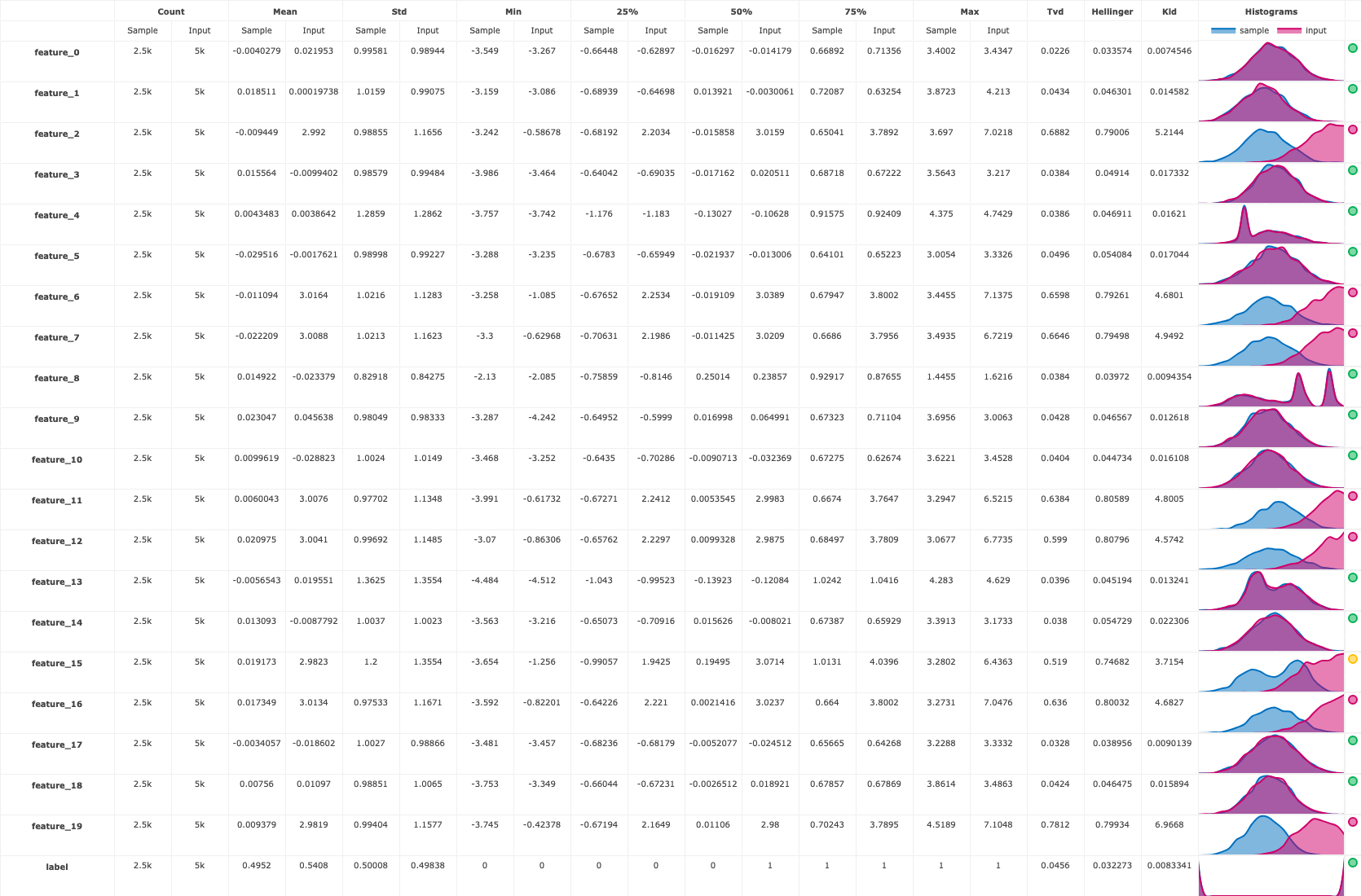
The custom histogram data drift model monitoring application you deployed provides additional plots like:
drift_table_plot that compares the drift between the training data and prediction data per feature;
and features_drift_results to show each feature drift score.
import time
import mlrun.model_monitoring.api

# Wait two minutes for the model monitoring applications flow to finish
time.sleep(120)

# Getting model endpoint
# Note: .to_job() auto-appends '-batch' suffix, so we use 'serving-fn-1-batch'
endpoint = mlrun.get_run_db().get_model_endpoint(
    name="my_model",
    function_name="serving-fn-1-batch",
    function_tag="latest",
    project=project.name,
    feature_analysis=True,
)

project.get_artifact(f"drift_table_plot-{endpoint.metadata.uid}").to_dataitem().show()
Finally, you also get a numerical drift metric and boolean flag denoting whether or not data drift is detected:
import mlrun.model_monitoring.api
import yaml

print(f"Drift detected : {'yes' if endpoint.status.result_status == 2 else 'no'}")
print(
    f"Drift metrics :\n{yaml.dump(endpoint.status.drift_measures, default_flow_style=False)}"
)
Drift detected : no
Drift metrics :
feature_0:
  hellinger: 0.0335736819532152
  kld: 0.008009146080386144
  tvd: 0.022800000000000008
feature_1:
  hellinger: 0.04630145403326306
  kld: 0.015136099233745433
  tvd: 0.04359999999999999
feature_10:
  hellinger: 0.04473407115760209
  kld: 0.01610759551132681
  tvd: 0.04039999999999998
feature_11:
  hellinger: 0.8058863402254881
  kld: 8.207418374913285
  tvd: 0.8432000000000001
feature_12:
  hellinger: 0.807957523155725
  kld: 8.5406740489432
  tvd: 0.8336
feature_13:
  hellinger: 0.04519449310948248
  kld: 0.014349562433429235
  tvd: 0.039999999999999994
feature_14:
  hellinger: 0.05472944756352956
  kld: 0.02230629686201226
  tvd: 0.038
feature_15:
  hellinger: 0.746815136758792
  kld: 7.493164579525917
  tvd: 0.7435999999999999
feature_16:
  hellinger: 0.8003245177804857
  kld: 8.097063905853084
  tvd: 0.8412
feature_17:
  hellinger: 0.038955714991485355
  kld: 0.010677448229097126
  tvd: 0.03320000000000001
feature_18:
  hellinger: 0.04647465218765195
  kld: 0.015894237456896398
  tvd: 0.04240000000000001
feature_19:
  hellinger: 0.7993397396310428
  kld: 7.613455815187319
  tvd: 0.8283999999999999
feature_2:
  hellinger: 0.7900559843329186
  kld: 7.404702739661648
  tvd: 0.8264
feature_3:
  hellinger: 0.04913963802970058
  kld: 0.017331946342858506
  tvd: 0.038400000000000004
feature_4:
  hellinger: 0.04691128230500036
  kld: 0.01676472797382658
  tvd: 0.03879999999999999
feature_5:
  hellinger: 0.05408439667581095
  kld: 0.02148043407690502
  tvd: 0.05039999999999999
feature_6:
  hellinger: 0.7926084404395208
  kld: 7.631668338501731
  tvd: 0.8400000000000002
feature_7:
  hellinger: 0.7949812589747411
  kld: 7.75413745622129
  tvd: 0.8368000000000001
feature_8:
  hellinger: 0.0397202637470994
  kld: 0.011098991721351776
  tvd: 0.03880000000000001
feature_9:
  hellinger: 0.046567270093498515
  kld: 0.014281787464135899
  tvd: 0.0432
hellinger_mean: 0.3581011459498972
kld_mean: 3.313215865571035
label:
  hellinger: 0.6357687578017881
  kld: 6.6518096447982895
  tvd: 0.4952
tvd_mean: 0.3599238095238095
# Data/concept drift per feature
import json

json.loads(
    project.get_artifact(f"features_drift_results-{endpoint.metadata.uid}")
    .to_dataitem()
    .get()
)
{'feature_0': 0.028186841,
 'feature_1': 0.044950727,
 'feature_2': 0.8082279922,
 'feature_3': 0.043769819,
 'feature_4': 0.0428556412,
 'feature_5': 0.0522421983,
 'feature_6': 0.8163042202,
 'feature_7': 0.8158906295,
 'feature_8': 0.0392601319,
 'feature_9': 0.044883635,
 'feature_10': 0.0425670356,
 'feature_11': 0.8245431701,
 'feature_12': 0.8207787616,
 'feature_13': 0.0425972466,
 'feature_14': 0.0463647238,
 'feature_15': 0.7452075684,
 'feature_16': 0.8207622589,
 'feature_17': 0.0360778575,
 'feature_18': 0.0444373261,
 'feature_19': 0.8138698698,
 'label': 0.5654843789}
Examining the drift results in the dashboard#
This section reviews the main charts and statistics that can be found on the platform dashboard. See Model monitoring architecture to learn more about the available model monitoring features and how to use them.
Before analyzing the results in the visual dashboards, run another batch infer job, but this time with drifted data, to get a drifted result. The drift decision rule is the value per-feature mean of the Total Variance Distance (TVD) and Hellinger distance scores.
In the histogram-data-drift application, the "Drift detected" threshold is 0.7 and the "Drift suspected" threshold is 0.3
fn = project.set_function(
    func="src/my_model.py", name="serving-fn-2", kind="serving", image="mlrun/mlrun"
)

graph = fn.set_topology("flow", engine="async")

model_runner_step = mlrun.serving.ModelRunnerStep(name="my_model_runner")

model_runner_step.add_model(
    model_class="MyModel",
    endpoint_name="my_drifted_model",
    model_artifact=model_artifact,
    execution_mechanism="naive",
    model_endpoint_creation_strategy=mm_constants.ModelEndpointCreationStrategy.OVERWRITE,
)

graph.to(model_runner_step).respond()
fn.set_tracking()
job = fn.to_job()

inputs = {"data": drifted_prediction_set_path}
run_obj = project.run_function(job, inputs=inputs)
> 2025-10-27 15:58:05,775 [info] Storing function: {"db":"http://mlrun-api:8080","name":"serving-fn-2-batch-execute-graph","uid":"8ae46fdf34d04af2b994c79399eb9239"}
> 2025-10-27 15:58:06,065 [info] Job is running in the background, pod: serving-fn-2-batch-execute-graph-rsdb5
> 2025-10-27 15:58:09,615 [info] Waiting for model endpoint creation task '0b1bb0d5-4761-48bc-95f4-fb729314c39d'...
> 2025-10-27 15:58:49,860 [info] Creating Model Monitoring stream target using uri:: {"uri":"ds://batch-stream/projects/tutorial-iguazio/model-endpoints/stream-v1"}
> 2025-10-27 15:58:49,879 [info] Initializing graph steps
> 2025-10-27 15:58:52,333 [info] Graph was initialized: {"verbose":false}
> 2025-10-27 15:58:58,736 [info] Job completed processing 2500 rows: {"model_endpoint_uids":["bf578e577beb4fcfb2fca4be3f6b2a6c"],"timestamp_column":null}
> 2025-10-27 15:58:58,954 [info] To track results use the CLI: {"info_cmd":"mlrun get run 8ae46fdf34d04af2b994c79399eb9239 -p tutorial-iguazio","logs_cmd":"mlrun logs 8ae46fdf34d04af2b994c79399eb9239 -p tutorial-iguazio"}
> 2025-10-27 15:58:58,954 [info] Or click for UI: {"ui_url":"https://dashboard.default-tenant.app.vmdev219.lab.iguazeng.com/mlprojects/tutorial-iguazio/jobs/monitor-jobs/serving-fn-2-batch-execute-graph/8ae46fdf34d04af2b994c79399eb9239/overview"}
> 2025-10-27 15:58:58,956 [info] Run execution finished: {"name":"serving-fn-2-batch-execute-graph","status":"completed"}
| project | uid | iter | start | end | state | kind | name | labels | inputs | parameters | results | artifacts |
|---|---|---|---|---|---|---|---|---|---|---|---|---|
| tutorial-iguazio | 0 | Oct 27 15:58:09 | 2025-10-27 15:58:58.944454+00:00 | completed | run | serving-fn-2-batch-execute-graph | v3io_user=iguazio kind=job owner=iguazio mlrun/client_version=0.0.0+unstable mlrun/client_python_version=3.9.22 host=serving-fn-2-batch-execute-graph-rsdb5 |
data |
num_rows=2500 |
prediction |
> 2025-10-27 15:59:02,578 [info] Run execution finished: {"name":"serving-fn-2-batch-execute-graph","status":"completed"}
Now you can observe the drift result:
time.sleep(120)

# Note: .to_job() auto-appends '-batch' suffix, so we use 'serving-fn-2-batch'
endpoint = mlrun.get_run_db().get_model_endpoint(
    name="my_drifted_model",
    function_name="serving-fn-2-batch",
    function_tag="latest",
    project=project.name,
    feature_analysis=True,
)

print(f"Drift detected : {'yes' if endpoint.status.result_status == 2 else 'no'}")
print(
    f"Drift metrics :\n{yaml.dump(endpoint.status.drift_measures, default_flow_style=False)}"
)
Drift detected : yes
Drift metrics :
feature_0:
  hellinger: 1.0
  kld: 15.947831766111843
  tvd: 1.0
feature_1:
  hellinger: 1.0
  kld: 15.942530740720343
  tvd: 1.0
feature_10:
  hellinger: 0.04473407115760209
  kld: 0.01610759551132681
  tvd: 0.04039999999999998
feature_11:
  hellinger: 0.8058863402254881
  kld: 8.207418374913285
  tvd: 0.8432000000000001
feature_12:
  hellinger: 0.807957523155725
  kld: 8.5406740489432
  tvd: 0.8336
feature_13:
  hellinger: 0.04519449310948248
  kld: 0.014349562433429235
  tvd: 0.039999999999999994
feature_14:
  hellinger: 0.05472944756352956
  kld: 0.02230629686201226
  tvd: 0.038
feature_15:
  hellinger: 0.746815136758792
  kld: 7.493164579525917
  tvd: 0.7435999999999999
feature_16:
  hellinger: 0.8003245177804857
  kld: 8.097063905853084
  tvd: 0.8412
feature_17:
  hellinger: 0.038955714991485355
  kld: 0.010677448229097126
  tvd: 0.03320000000000001
feature_18:
  hellinger: 0.04647465218765195
  kld: 0.015894237456896398
  tvd: 0.04240000000000001
feature_19:
  hellinger: 0.7993397396310428
  kld: 7.613455815187319
  tvd: 0.8283999999999999
feature_2:
  hellinger: 1.0
  kld: 15.954249871425905
  tvd: 1.0
feature_3:
  hellinger: 1.0
  kld: 16.040915135106705
  tvd: 1.0
feature_4:
  hellinger: 1.0
  kld: 16.070032712370534
  tvd: 1.0
feature_5:
  hellinger: 1.0
  kld: 15.853046186129449
  tvd: 1.0
feature_6:
  hellinger: 1.0
  kld: 15.892588362525855
  tvd: 1.0
feature_7:
  hellinger: 1.0
  kld: 15.9013904377493
  tvd: 1.0
feature_8:
  hellinger: 1.0
  kld: 15.935217661233796
  tvd: 1.0
feature_9:
  hellinger: 1.0
  kld: 15.965031755202492
  tvd: 1.0
hellinger_mean: 0.7040958620235437
kld_mean: 9.772022874285877
label:
  hellinger: 0.5956014659331326
  kld: 5.678533866511663
  tvd: 0.4952
tvd_mean: 0.7037714285714287
Model Endpoints#
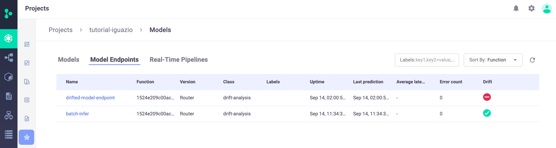
In the Projects page > Model endpoint summary list, you can see the new two model endpoints, including their drift status:
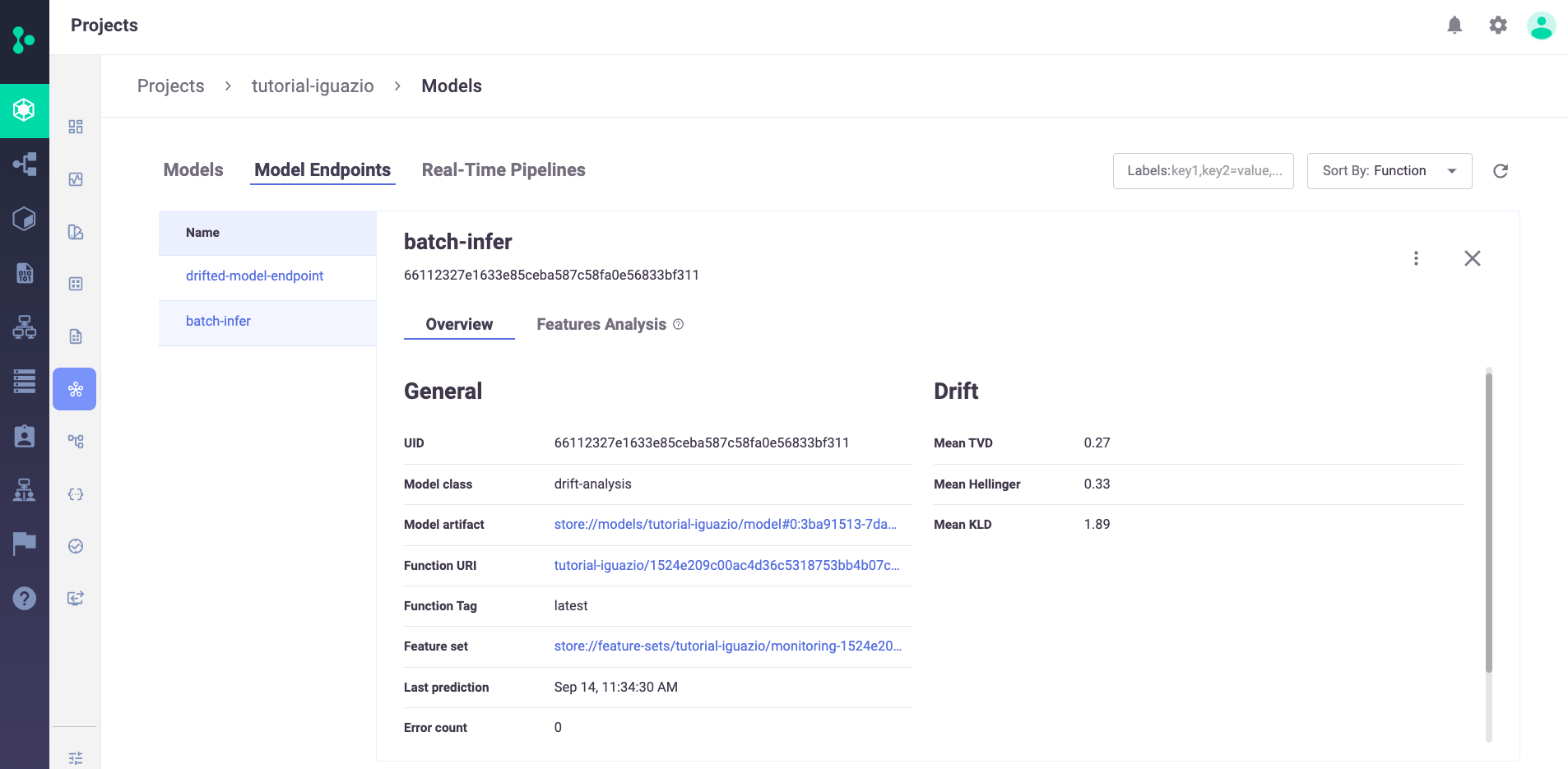
You can zoom into one of the model endpoints to get an overview about the selected endpoint, including the calculated statistical drift metrics:
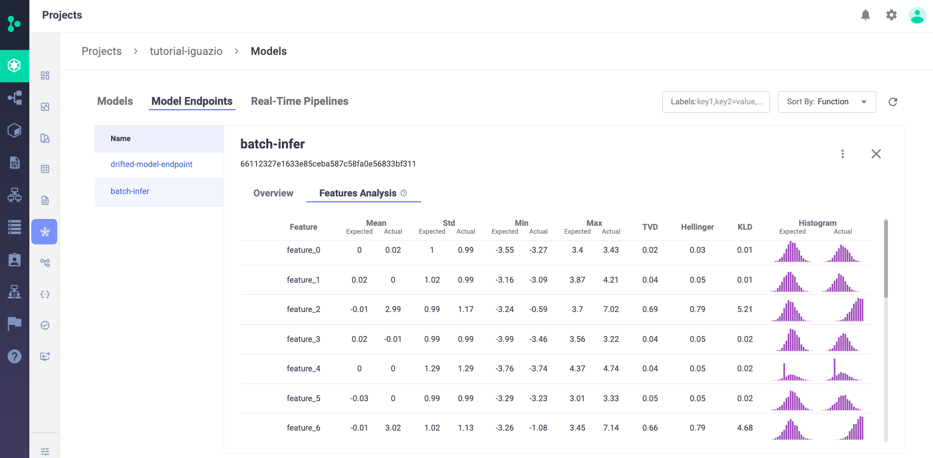
Press Features Analysis to see details of the drift analysis in a table format with each feature in the selected model on its own line, including the predicted label:
Next steps#
In a production setting, you probably want to incorporate this as part of a larger pipeline or application.
For example, if you use this function for the prediction capabilities, you can pass the prediction output as the input to another pipeline step, store it in an external location like S3, or send to an application or user.
If you use this function for the drift detection capabilities, you can use the drift_status and drift_metrics outputs to automate further pipeline steps, send a notification, or kick off a re-training pipeline.
Done!#
Congratulations! You've completed Part 6 of the MLRun getting-started tutorial. You may want to review the additional tutorials: