Batch inference

Batch inference or offline inference addresses the need to run machine learning model on large datasets. It is the process of generating outputs on a batch of observations.

With batch inference, the batch runs are typically generated during some recurring schedule (e.g., hourly, or daily). These inferences are then stored in a database or a file and can be made available to developers or end users. With batch inference, the goal is usually tied to time constraints and the service-level agreement (SLA) of the job. Conversely, in real time serving, the goal is usually to optimize the number of transactions per second that the model can process. An online application displays a result to the user.

Batch inference can sometimes take advantage of big data technologies, such as Spark, to generate predictions. Big data technologies allow data scientists and machine learning engineers to take advantage of scalable compute resources to generate many predictions simultaneously. To gain a better understanding about the batch inference usage and the function parameters, see the Batch Inference page on the Function Hub.

Test your model

To evaluate batch model prior to deployment, you should use the evaluate handler of the auto_trainer function.

This is typically done during model development. For more information refer to the Evaluate handler documentation. For example:

import mlrun

# Set the base project name
project_name_base = 'batch-inference'

# Initialize the MLRun project object
project = mlrun.get_or_create_project(project_name_base, context="./", user_project=True)

auto_trainer = project.set_function(mlrun.import_function("hub://auto_trainer"))

evaluate_run = project.run_function(
    auto_trainer,
    handler="evaluate",
    inputs={"dataset": train_run.outputs['test_set']},
    params={
        "model": train_run.outputs['model'],
        "label_columns": "labels",
    },
)

Deploy your model

Batch inference is implemented in MLRun by running the function with an input dataset. With MLRun you can easily create any custom logic in a function, including loading a model and calling it.

The Function Hub batch inference function is used for running the models in batch as well as performing drift analysis. The function supports the following frameworks:

• Scikit-learn

• XGBoost

• LightGBM

• Tensorflow/Keras

• PyTorch

• ONNX

Internally the function uses MLRun's out-of-the-box capability to load run a model via the mlrun.frameworks.auto_mlrun.auto_mlrun.AutoMLRun class.

Basic example

The simplest example to run the function is as follows:

Create project

Import MLRun and create a project:

import mlrun

project = mlrun.get_or_create_project(
    "batch-inference", context="./", user_project=True
)
batch_inference = mlrun.import_function("hub://batch_inference_v2")

Get the model

Get the model. The model is a decision tree classifier from scikit-learn. Note that if you previously trained your model using MLRun, you can reference the model artifact produced during that training process.

import sys

suffix = (
    mlrun.__version__.split("-")[0].replace(".", "_")
    if sys.version_info[1] > 7
    else "3.7"
)

model_path = mlrun.get_sample_path(f"models/batch-predict/model-{suffix}.pkl")

model_artifact = project.log_model(
    key="model", model_file=model_path, framework="sklearn"
)

Get the data

Get the dataset to perform the inference. The dataset is in parquet format.

prediction_set_path = mlrun.get_sample_path("data/batch-predict/prediction_set.parquet")

Run the batch inference function

Run the inference. In the first example we will not perform any drift analysis

batch_run = project.run_function(
    batch_inference,
    inputs={"dataset": prediction_set_path, "model_path": model_artifact.uri},
)

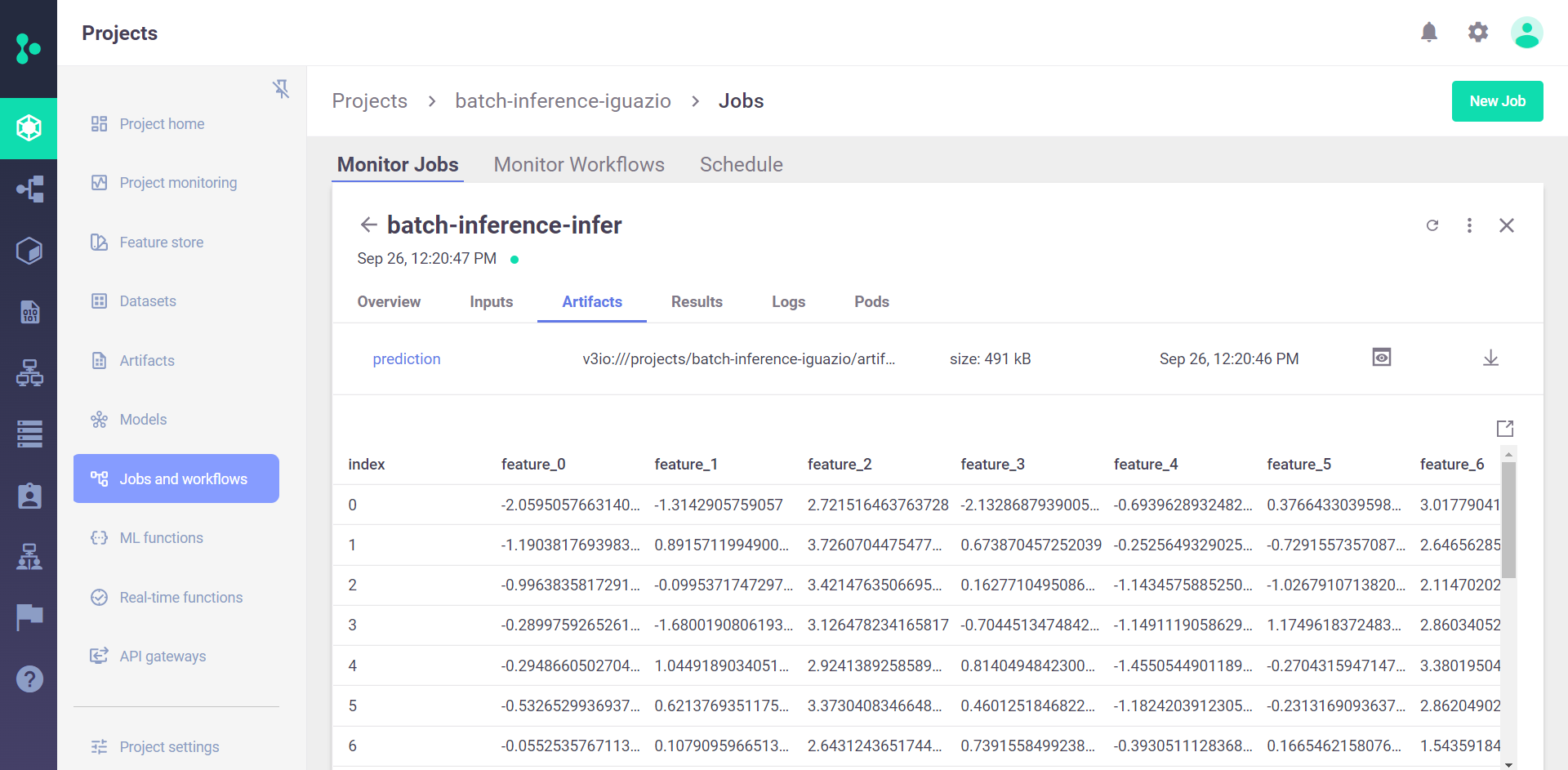
Function output

The output of the function is an artifact called prediction:

batch_run.artifact("prediction").as_df().head()

	feature_0	feature_1	feature_2	feature_3	feature_4	feature_5	feature_6	feature_7	feature_8	feature_9	...	feature_11	feature_12	feature_13	feature_14	feature_15	feature_16	feature_17	feature_18	feature_19	predicted_label
0	-2.059506	-1.314291	2.721516	-2.132869	-0.693963	0.376643	3.017790	3.876329	-1.294736	0.030773	...	2.775699	2.361580	0.173441	0.879510	1.141007	4.608280	-0.518388	0.129690	2.794967	0
1	-1.190382	0.891571	3.726070	0.673870	-0.252565	-0.729156	2.646563	4.782729	0.318952	-0.781567	...	1.101721	3.723400	-0.466867	-0.056224	3.344701	0.194332	0.463992	0.292268	4.665876	0
2	-0.996384	-0.099537	3.421476	0.162771	-1.143458	-1.026791	2.114702	2.517553	-0.154620	-0.465423	...	1.729386	2.820340	-1.041428	-0.331871	2.909172	2.138613	-0.046252	-0.732631	4.716266	0
3	-0.289976	-1.680019	3.126478	-0.704451	-1.149112	1.174962	2.860341	3.753661	-0.326119	2.128411	...	2.328688	3.397321	-0.932060	-1.442370	2.058517	3.881936	2.090635	-0.045832	4.197315	1
4	-0.294866	1.044919	2.924139	0.814049	-1.455054	-0.270432	3.380195	2.339669	1.029101	-1.171018	...	1.283565	0.677006	-2.147444	-0.494150	3.222041	6.219348	-1.914110	0.317786	4.143443	1

5 rows × 21 columns

View the results in the UI

The output is saved as a parquet file under the project artifact path. In the UI you can go to the batch-inference-infer job --> artifact tab to view the details.

Scheduling a batch run

To schedule a run, you can set the schedule parameter of the run method. The scheduling is done by using a cron format.

You can also schedule runs from the dashboard. On the Projects > Jobs and Workflows page, you can create a new job using the New Job wizard. At the end of the wizard, you can set the job scheduling. In the following example, the job is set to run every 30 minutes.

batch_run = project.run_function(
    batch_inference,
    inputs={"dataset": prediction_set_path, "model_path": model_artifact.uri},
    schedule="*/30 * * * *",
)

Drift analysis

By default, if a model has a sample set statistics, batch_inference performs drift analysis and produces a data drift table artifact, as well as numerical drift metrics. In addition, this function either creates or updates an existing model endpoint record (depends on the provided endpoint_id).

In addition, you can define "trigger_monitoring_job": True to trigger the drift job analysis immediately.

To provide sample set statistics for the model you can either:

1. Train the model using MLRun. This allows you to create the sample set during training.

2. Log an external model using project.log_model method and provide the training set in the training_set parameter.

3. Provide the set explicitly when calling the batch_inference function via the model_endpoint_sample_set input.

In the example below, we will provide the training set as the sample set

training_set_path = mlrun.get_sample_path("data/batch-predict/training_set.parquet")

batch_run = project.run_function(
    batch_inference,
    inputs={
        "dataset": prediction_set_path,
        "model_endpoint_sample_set": training_set_path,
        "model_path": model_artifact.uri,
    },
    params={
        "label_columns": "label",
        "perform_drift_analysis": True,
        "trigger_monitoring_job": True,
    },
)

In this case, instead of just prediction, you get drift analysis. If no label column was provided, the job function tries to retrieve the label columns from the logged model artifact. If also not defined in the model, the label columns are generated with the following format predicted_label_{i} where i is an incremental number.

The drift table plot that compares the drift between the training data and prediction data per feature:

batch_run.artifact("drift_table_plot").show()

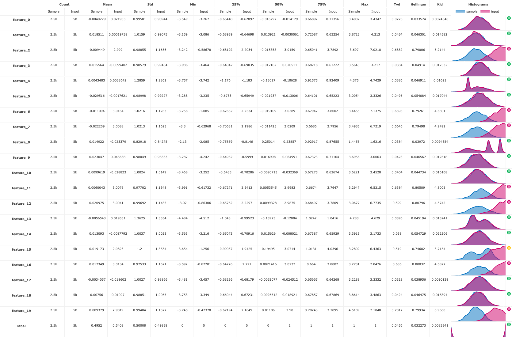
You also get a numerical drift metric and boolean flag denoting whether or not data drift is detected:

print(batch_run.status.results)

{'drift_status': False, 'drift_metric': 0.29934242566253266}

# Data/concept drift per feature (use batch_run.artifact("features_drift_results").get() to obtain the raw data)
batch_run.artifact("features_drift_results").show()

{'feature_0': 0.028086840976606773,
 'feature_1': 0.04485072701663093,
 'feature_2': 0.7391279921664593,
 'feature_3': 0.043769819014849734,
 'feature_4': 0.042755641152500176,
 'feature_5': 0.05184219833790496,
 'feature_6': 0.7262042202197605,
 'feature_7': 0.7297906294873706,
 'feature_8': 0.039060131873550404,
 'feature_9': 0.04468363504674985,
 'feature_10': 0.042567035578799796,
 'feature_11': 0.7221431701127441,
 'feature_12': 0.7034787615778625,
 'feature_13': 0.04239724655474124,
 'feature_14': 0.046364723781764774,
 'feature_15': 0.6329075683793959,
 'feature_16': 0.7181622588902428,
 'feature_17': 0.03587785749574268,
 'feature_18': 0.04443732609382538,
 'feature_19': 0.7902698698155215,
 'label': 0.017413285340161608}